


Long-run restrictions are imposed on the matrix A=C*B. The matrix B contains the parameters of the contemporaneous effects of the structural shocks, while the C matrix is given in Johansen (1996) under unit roots. If there are no unit roots then the C matrix is simply the inverse of the reduced form VAR lag polynomial matrix evaluated at 1. That is, if the model is given by:
![]()
where xt is the vector of endogenous variables in levels, L is the lag operator such that Lxt = xt-1, and ηt are the structural shocks, then C = Π(1)-1 under the no unit root assumption. For this model A measures the accumulated effects of the structural shocks in the long-run. In contrast, for the unit root case A measure the effects of the structural shocks in the long-run.
The case of no unit roots generally doesn't imply any difficulties in setting up restrictions for A since it always has full rank for a given sample when the parameters of Π(L) are estimated freely. When there are unit roots we know that A has reduced rank and this limits the type of restrictions we can impose on it since we are not allowed to violate the rank condition.
Suppose we have a VAR model for 5 endogenous variables and the system is subject to 3 unit roots, i.e. 2 cointegration relations. This means that A has rank 3 since C has rank 3. Furthermore, let us assume that the form of the A matrix we wish to achieve can be described by the following (where * indicates any real number);
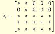
The upper left 2x2 matrix of this form for A will always have full rank when the first 2 variables in the system are both I(1). This means that the lower right 3x3 matrix must have rank 1. At the same time all the entries in this 3x3 matrix may be non-zero.
This model is thus subject to 3 common trends, where the first is given by the accumulation of the first structural shock, the second common trend by the accumulation of the second structural shock, and the third common trend is given by a linear combination of the last 3 structural shocks.
We can represent the lower right 3x3 matrix by:
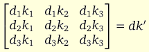
where the vectors d = [d1 d2 d3]' and k = [k1 k2 k3]' must both be non-zero. Hence we can think of the 3rd common trend as being the linear combination of the last 3 structural shocks determined by the vector [k1 k2 k3].
To achieve exact identification we need to impose 3 more restrictions on the model. Given that we're satisfied with the above form for A we can't yet separate out the effects of the last 3 structural shocks. In SVAR you're then restricted to imposing the remaining identifying assumptions on the B matrix.
An example of exact identification would be to use the following form for B (given A above):
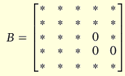
Among the last 3 shocks we now find that only the first of them is allowed to have a contemporaneous effect on the 4th variable, while only the second of them is not allowed to have a contemporaneous effect on the 3rd variable.