


The Markov switching test due to Carrasco, Hu and Ploberger (2004) can be computed by SVAR. Relative to other tests for Markov switching, the test by Carrasco et al. has the advantage that the model only has to be estimated under the null hypothesis of no Markov switching regimes. Since the asymptotic distribution depends on nuisance parameters, Carrasco et al suggest using parametric bootstrapping for inference. SVAR makes this possible from the Markov Switching Test dialog.
The user can influence a number of features of the test. First of all, the parameters that may be subject to a 2-state Markov switching process can be selected. The parameters are divided into 3 groups for this purpose: (i) the δ parameters (all deterministic variables but those restricted to the cointegration space); (ii) The α & Γ parameters (all parameters on stochastic variables); and (iii) the Ω parameters (residual covariances). Any combination of these 3 groups can be selected.
Furthermore, 2 sets of nuisance parameters need to be evaluated. These are given by a vector h and the parameter ρ, where the latter measures the autocorrelation of the Markov process. The vector h specifies the direction of the alternative and thus has the same dimension as the number of parameters that are allowed to vary with the Markov process under the alternative. This vector is an elements of the unit sphere.
When computing the test, a range of autocorrelation values are considered. This range can be selected by the user. Furthermore, rather than maximizing the expression of the test statistic over all h vectors for a given ρ, SVAR draws h uniformly from the unit sphere as many times as desired. This is typically faster than determining h numerically.
When bootstrapping the Markov Switching test, all Common Features are supported. In addition to these, the following parameters can be edited:
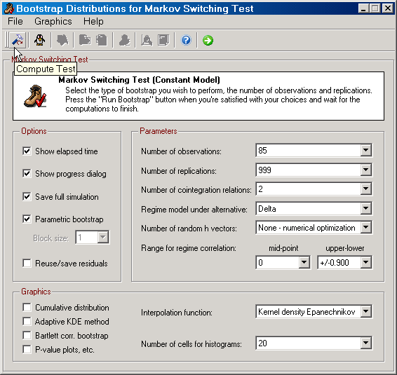
| • | Regime model under the alternative: Selects the parameter that can vary with the Markov switching process. |
| • | Number of random h vector: The number of draws from the uniform distribution over the unit sphere. By default, SVAR uses numerical optimization when choosing h. |
| • | Range for regime correlation: The user can determine the mid-point and the upper and lower bounds relative to the mid-point for this parameter. |
Furthermore, there is a Compute Test function in case you just want to calculate the test value.
|
Figure: The dialog for bootstrapping and computing the Markov switching test. |
The Test Statistic
The test statistic is constructed as follows:
sup TS = supρ, h: h'h = 1, ρ(l) <= ρ <= ρ(u) (1/2)*max{ 0, ΓΤ / √[(1/T) εε'] }2
where ρ(l) and ρ(u) give the lower and upper bounds for ρ, respectively, and T the sample size. The scalar ΓT and 1xT vector ε are computed as follows. Let ft be the vector of partial derivatives of the log data density for time period t with respect to the parameters that are allowed to change with the regime under the alternative, while Ht is the matrix of second order partials with respect to the same group of parameters. Furthermore, let Ft be the vector of partial derivatives of the log data density for time period t with respect to all parameters (except β), while μ2,t be given by
μ2,t = h' [ Ht + ftft' + 2 Σs=1 t-1 ρs ftft-s' ] h
Now,
ΓT = (1/2√T ) Σt=1 T μ2,t
while ε contains the residuals from the regression of (1/2)*μ2,t on Ft. Notice that ft, Ft and Ht are all evaluated under the parameter estimates under the null of no Markov switching. Moreover, the scalar c in Carrasco et al (2004), specifying the amplitude of the change, is cancelled out. This is the reason why h is restricted to the unit sphere.