


Most selections you can make on these dialogs are common across all dialogs. On each dialog you will see 3 frames with the headers Options, Parameters, and Graphics. The controls in the first two frames directly influence the bootstrap run. For example, "Parametric bootstrap" is located in the "Options" frame. When selected, SVAR performs a parametric bootstrap, as explained above, and when de-selected a non-parametric bootstrap. The controls in the "Graphics" frame influence the way SVAR displays graphs of the empirical bootstrap distributions. For example, if "Cumulative distribution" is selected, then SVAR displays cumulative distribution functions only, and when de-selected it displays the density functions. In addition, most toolbar buttons and menu options are common across all 7 bootstrap dialogs. Below follows 5 lists. Notice that most of the features on the File Menu and all of the features on the Graphics Menu are also displayed as push buttons on the toolbar of each dialog.
File Menu
| • | Run Bootstrap: Begins the bootstrap run. Available on the Toolbar. |
| • | Save to mat-file: Save bootstrapped statistics (tests and parameters) to Matlab MAT Files. These can then easily be loaded on the fly by SVAR. Available on the Toolbar. |
| • | Simulation Summary: Displays a dialog with summary statistics of the currently loaded (if any) bootstrap simulation. Available on the Toolbar. |
| • | Full Simulation: Display a dialog with most of the simulated statistics ordered from the smallest to the largest. Available on the Toolbar. |
| • | Append to Output: Allows you to append the simulation summary to the output file. The format used of the simulation summary (plain text or LaTeX) depends on which format you have selected for saving to the output file. |
| • | Center Window: Centers the dialog window. |
| • | Return: Returns to the previous dialog. Available on the Toolbar. |
Graphics Menu
| • | Graph Bootstrap Sample: Opens a dialog from which you can review the bootstrapped series for all replications. Requires that you have selected to "Reuse/save residuals to disk" on the "Options" dialog. Available on the Toolbar. |
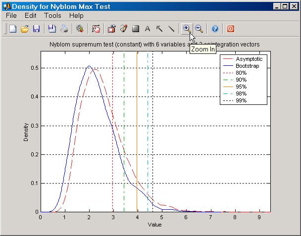
| • | Graph Distributions: Presents plots of the empirical densities or cumulative distributions of the bootstrapped test statistics and parameters that are currently loaded into memory. Available on the Toolbar. The Figure below gives an example of how SVAR presents plots of such bootstrapped distributions. |
|
Figure: Plot of asymptotic and bootstrapped distributions of the Nyblom supremum test. |
| • | Histogram of Distributions: Presents plots of with histograms of the above mentioned distributions. The selected "Number of cells for graphs" on the "Graphics" frame influence how many cells the histograms contain. Available on the Toolbar. |
Help Menu
| • | Help Topics: Opens the SVAR Help. On Windoze it will also open the help file at the Bootstrapping section. Available on the Toolbar. |
Options
| • | Show elapsed time: Presents the elapsed time since the bootstrap run was started on the progress dialog. Requires that the next check box has been selected. |
| • | Show progress dialog: Displays a progress dialog rather than just a wait dialog. Slows down the bootstrap runs, but gives you an idea of how much longer you have to wait until the bootstrap run has finished. |
| • | Save full simulation: Automatically saves all bootstrapped statistics to a Matlab MAT File after the bootstrap run has finished. Allows old bootstrap runs to be automatically loaded by SVAR if the parameters and options match. |
| • | Parametric bootstrap: Draws residuals from the Gaussian distribution rather than from the estimated residuals when computing bootstrapped data series. |
| • | Block size: When the parametric bootstrapping checkbox is not check marked, SVAR can perform block bootstraps. The size of the block length determines how large the blocks are, with values greater than 1 implying a block bootstrap. |
| • | Reuse/save residuals: Saves the bootstrapped residuals to disk and unsorted test statistics. The bootstrapped residuals can then later be reused to re-run the bootstrap. |
Parameters
| • | Number of observations: Allows you to select the number of observations in each bootstrapped data series. Defaults to the same number as the original data series, but may be changed if you have selected to run a parametric bootstrap. Selecting a different number of observations than for the original data series makes it possible to check, e.g., how quickly the empirical distribution of a test statistic converges to the asymptotic. |
| • | Number of replications: Determines how many bootstrap samples to compute. The seemingly odd numbers that can be selected (99, 999, etc) stem from the simple observation that in order to get, e.g., an empirical size right the selected level times the number of bootstrap replications plus one must be an integer. This is most easily understood by considering the number of possible outcomes when comparing an original test to its empirical bootstrap distribution. If we have 99 replications, the number of bootstrapped tests that can be greater than the original statistic is 0, 1, ... , 99. That is, 100 possible outcomes; see, e.g., Davidson and MacKinnon (2000a) for details. |
| • | Number of cointegration relations: Allows you to change (in some cases) the number of cointegration relations for the model you're using. |
Graphics
| • | Cumulative distribution: By default SVAR plots empirical density functions from the bootstrap when graphing distributions. By check marking this box it will graph cumulative distributions instead. |
| • | Adaptive KDE methods: Whenever the selected interpolation function (see below) is a Kernel density estimator, you can select the adaptive version of the estimator instead. |
| • | Bartlett corr. bootstrap: When available SVAR can estimate the Bartlett correction factor based on the empirical distribution by simply calculating the average and comparing it to the mean of the asymptotic distribution. When plotting test distributions it will then add a "Bartlett corrected" empirical distribution along with the empirical and the asymptotic. This option is not available on the Trace Distribution and Nyblom Distribution dialogs. In the former case you can tell SVAR to compute Bartlett corrected trace tests on the Cointegration tab on the Preferences dialog. In the latter case, the asymptotic distributions are currently not available to SVAR. When they are, this option will appear on that dialog. |
| • | P-value plots, etc: When graphing distributions of bootstrapped tests SVAR can compute several type of PP and QQ plots. By check marking this option, such plots will be provided; see Davidson and MacKinnon (1998) for details on computations. |
| • | Interpolation function: When graphing distributions of tests and other parameters, SVAR can use 12 different methods for computing densities and cumulative distributions. You can influence the default choice on the Simulation tab on the Preferences dialog. If you change you're mind after you've run your bootstrap, the interpolation function can also be changed on the fly. |
| • | Number of cells for histograms: This option allows you to choose how many bars to show in a histogram of an empirical distribution. |