


The Bayesian analysis performed through SVAR is based on either informative or non-informative priors for the parameters of interest. By default, non-informative priors are used for the short-run dynamics and the parameters on deterministic variables. For α, β, and Ω the default is an informative prior on α|β,Ω, a uniform prior on the space spanned by β, and an informative prior on Ω. This can be changed to informative priors on the Bayesian tab on the Preferences dialog.
When an informative prior is selected for the short-run dynamics then a Gaussian prior is used conditional on Ω. This includes the parameters on first differences of exogenous I(1) variables and the levels of exogenous I(0) variables. Similarly, a Gaussian prior distribution conditional on Ω is used for the parameters on any deterministic variables given that these parameters are not restricted to the cointegration relations. For α|β,Ω a Gaussian distribution is also used. For the reduced form residual covariance matrix an inverted Wishart distribution is used, while the default prior for the cointegration rank assigns equal probabilities to all possible ranks. The model parameters are assumed to be independent conditional on Ω across the groups short-run dynamics, deterministics, (α, β), and the cointegration rank.
The prior distributions can be changed on the Bayesian tab on the Preferences dialog. It is also possible to select non-informative priors on this dialog, but this only affects the short-run parameters and the deterministics when the analysis concerns the cointegration rank.
I. Error Correction Model
The prior distribution for the short-run dynamics is given by:
vec(Γ,Φ,Ψ) | Ω ~ N(μΓ,Φ,Ψ, ΣΓ,Φ,Ψ ⊗ Ω),
where μΓ,Φ,Ψ = E[vec(Γ), vec(Φ), vec(Ψ)], Γ = [Γ1 ... Γk-1], Φ = [Φ0 .. Φm], and Ψ = [Ψ0 ... Ψm-1]. The Φi matrices appear on the levels of exogenous I(0) variables, and the Ψj matrices on the first differences of exogenous I(1) variables. The parameter p is the lag length for the endogenous variables in the VAR model, while m is the lag length for the exogenous variables. If m=0 then Ψ is an empty matrix. When the variances of the parameters are finite the prior is said to be informative (and proper). A non-informative (improper) prior has infinite variances.
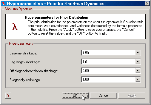
The prior distribution for the short-run dynamics has zero mean (μΓ,Φ,Ψ = 0) and co-variances determined by a structured shrinkage expression. Specifically:
Σ(Γi) = [ (λb)2 / i2λl ] In,
where In is the nxn identity matrix. The hyperparameter λb measures the baseline shrinkage. The lag length shrinkage hyperparameter λl measures how quickly the lag parameters decay.
It is also possible to allow for correlation between Γi and Γj. The is handled through the off-diagonal/correlation shrinkage hyperparameter. Here,
Σ(Γi,Γj) = [λρ (λb)2 / iλl jλl (i-j)2] In.
For parameters on first differences of exogenous I(1) variables and levels of exogenous I(0) variables, SVAR multiplies an exogeneity shrinkage hyperparameter λe to the power of 2 to the above expressions for i=1, 2, etc.
|
Figure: The dialog for editing the prior hyperparameters for the short-run dynamics. |
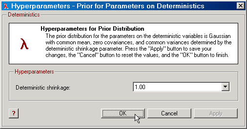
Let δ denote the matrix with parameters on deterministic variables. The prior distribution for these parameters is given by:
vec(δ) | Ω ~ N( μδ, Σδ ⊗ Ω ),
where μδ = E[vec(δ)] = 0. The covariance matrix for these parameters is given by:
Σδ = (λd)2 Id,
where Id is the d-dimensional identity matrix. The hyperparameter λd is called the deterministic shrinkage.
This prior can potentially be improved upon by using the ideas presented in Villani (2007). The prior discussed by Villani (2007) takes into account that the mean growth rates and the mean of the cointegration relations are functions of the δ parameters. Using such information can potentially lead to a the formulation of a "better" prior for δ. Such a feature may be included in SVAR at a later stage.
|
Figure: The dialog for editing the deterministic shrinkage hyperparameter in SVAR. |
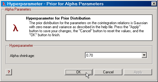
The prior distribution for α, the parameters on the cointegration relations, is directly taken from Villani (2005b). This prior is conditional on β, the cointegration space, and Ω, where Ω is the covariance matrix for the residuals. It states that
vec(α)|β, Ω ~ N(0, Σα),
where
Σα = [(β'*β)-1 ⊗ (λα)2 )*Ω].
The α shrinkage hyperparameter λα takes on positive values between 0 and 10000 and the default value is 10. See Strachan and Inder (2004) and Villani (2005b) for a motivation for this prior.
NOTE: The value of λα is closely related to the scale of the endogenous variables. For example, suppose all endogenous variables are measured in percent. A value of λα=1 may then be considered appropriate. If the same data is now divided by 100, then a value of λα=100 implies the same prior distribution as before given that the prior of Ω is unaffected.
|
Figure: The dialog for editing the α shrinkage hyperparameter in SVAR. |
Beta
The prior distribution for β is based on the reference prior in Villani (2005b). That is, we use a prior for β that implies that the span of β, denoted by sp(β), is uniformly distributed over the Grassman manifold of dimension r,n-r, where n is the number of endogenous variables. SVAR currently uses the familiar parameterization
β = β(c'β)-1
where c is taken from r columns of the n-dimensional identity matrix. SVAR examines all such matrices and chooses the one which results in the largest absolute value of the determinant of c'*( diag(Ω)1/2)*β, where diag(A) is the diagonal of a square matrix. For some drawbacks with this prior, see, e.g., Strachan and Inder (2004). In the future, different priors and parameterizations of the cointegration space will be supported by SVAR.
For this parameterization of the cointegration space, the prior can be formulated as
p(β|r) is proportional to det(β'β)-n/2
where n is the number of endogenous variables. Generally, we may think of this prior as assigning equal probability to every possible cointegration space of dimension r when the cointegration relations are exactly identified and there are no restrictions on α (as is the case when the Bayesian cointegration rank analysis is performed).
When specific identifying linear restrictions have been imposed on the cointegration space, the elements of β may be mapped into the free parameters according to
vec(β) = h + H*ϕ
The prior is still formulated as
p(β|r) ∝ det(β'β)-n/2
For models with a restricted constant/linear trend and models with exogenous I(1) variables we assign the same prior but it may be inappropriate for such models (as suggested by Mattias Villani in personal communication). It is nevertheless used by SVAR until a more appropriate prior is presented in the literature.
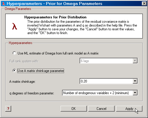
When investigating the cointegration rank it is necessary (see, e.g., Villani, 2005b) to use an informative prior for Ω. SVAR uses the following prior for Ω in this case:
p(Ω) ~ IW(A,q)
where A is either given by the maximum likelihood estimate of Ω for the model with full cointegration rank (and a selected lag order) or a scalar times the identity matrix. This scalar is another hyperparameter called the A matrix shrinkage by SVAR. The parameter q is by default equal to n+2, where the integer n is the dimension of Ω, and IW(A,q) denotes the inverted Wishart distribution with mean A and q degrees of freedom; see Zellner (1971) for definitions and properties of this distribution. Values of q greater than n+2 can also be selected. This prior is always used when investigating the cointegration rank.
The matrix A can be selected in two different ways. First, the maximum likelihood estimate of Ω can be used for a full rank model with a certain value for k, the lag order. In this case, q is always equal to n+2. Alternatively, the A matrix can be set according to
A = λA In
where λA is a positive scalar. In this case, the q parameter can be selected from a range of different values, with a minimum of n+2 and a maximum of T, the sample size.
The prior distribution for the reduced form residual covariance parameters can otherwise (for fixed cointegration rank) be given by the common diffuse prior. That is:
p(Ω) ∝ det(Ω)-(n+1)/2.
This means that the full conditional posterior for Ω is the usual inverted Wishart; see Zellner (1971) for details.
|
Figure: The dialog for editing the Ω prior in SVAR. |
The Full Prior Conditional on the Cointegration Rank
Given the above we thus have that the full prior for the cointegrated VAR model with r cointegration relations is:
p(Γ,Φ,Ψ, δ, α, β, Ω|r) = p(Γ|Ω)*p(Φ|Ω)*p(Ψ|Ω)*p(δ|Ω)*p(α|β, Ω, r)*p(β|r)*p(Ω)
II. VAR Models in Levels
If you have opted for No Cointegration Estimation on the Parameters tab on the main program window, the Bayesian analysis is carried out in a VAR model in levels. Since the parameters in a levels VAR are different from those of the same model written on error correction form, the prior is constructed in a slightly different way. The parameters on the deterministic variables and those forming the covariance matrix of the residuals, however, are the same across the two representations. Hence, SVAR uses exactly the same specification for the priors for these parameters.
The main difference for the levels VAR relative to the error correction form concerns the parameters on lagged endogenous variables and those on exogenous stochastic variables. The prior for the levels VAR is identical to the prior for the error correction model for the short-run dynamics when it comes to the prior variances. Moreover, the prior mean is the same across these two models for the parameters on the exogenous stochastic variables. The main difference is for the prior mean of the parameters on lagged endogenous. SVAR here applies the Minnesota mean for the prior. That is, all diagonal elements of the matrix on the first lag of the endogenous variables have unit prior mean. All other parameters on lagged endogenous variables have zero mean. Hence, the "prior expectation" for the endogenous variables is that the current value is equal to the previous.