If you have opted for conducting a Bayesian analysis of your VAR model, clicking on the "Analyse Model" button on the Main Program window takes you to the Bayesian Analysis dialog. In contrast to the Classical Analysis GUI, all Bayesian analysis is conducted from the same dialog.
|
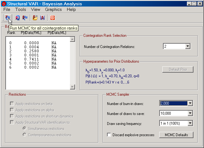
Figure: The Bayesian analysis dialog in SVAR.
|
The Bayesian analysis dialog contains 5 menus, a toolbar, and various information and selection controls. The upper left corner displays information about cointegration rank. The number of potential ranks is equal to n+1, where n is the number of endogenous variables in the cointegrated VAR model. Initially, this information control also displays the posterior cointegration rank probabilities, calculated from the fractional marginal likelihood (FML); see Corrander and Villani (2004) for details on how these are determined. Once the Bayesian cointegration analysis based on the marginal likelihood (ML) has been undertaken, the posterior rank probabilities based on these statistics will also be displayed. Prior to such analysis, these probabilities are represented by NA.
The upper right corner shows the cointegration rank selection control. Given that "Cointegration Estimation" has been selected on the Parameters tab of the Main Program window, this control is enabled, allowing you to choose a rank between 0 and n.
The frame in the middle right part presents information about the selected hyperparameters of the prior distributions. If you have made any changes to these parameters from Tools menu, the "Default Prior" button will be enabled. Clicking this button resets all such hyperparameters to their default values. The default values can be changed permanently on the Bayesian tab on the Preferences dialog.
The frame in the lower left corner provides an opportunity to, given the cointegration rank, select a model with specific restrictions. These controls will only be enabled once sampling from the posterior distribution has been conducted from the model.
The controls in the frame in the lower right corner all concern properties of the Markov Chain Monte Carlo (MCMC) sampler. All these controls have default values that are set on the Bayesian tab of the Preferences dialog. Since you may be interested in temporarily using other values than the defaults, you can edit the "Number of burn-in draws", the "Number of draws to save", the "Draw saving frequency", and whether or not to discard draws from the posterior that imply an explosive process. If you have changed the default value of one of these MCMC sampler parameters, the "MCMC Defaults" button is enabled, allowing you to quickly reset the controls back to their default values.
The cointegration rank analysis is based on the work by Villani (2005b).
File Menu
| • | Beta: Run the Gibbs sampler for the model with specific restriction on β given a cointegration rank between 1 and n-1. This function is also available on the Toolbar. |
| • | Cointegration Rank: Run the Gibbs sampler for all cointegration ranks. Once this function has been completed, the marginal likelihood can be determined and therefore also the posterior cointegration rank probabilities. This function is also available on the Toolbar. |
| • | Beta: Opens the Beta restrictions dialog. This function is also available on the Toolbar. |
| • | Open Beta Restrictions: Opens a dialog where you can choose previously saved beta restriction from file. This function is also available on the Toolbar. |
| • | Save Beta Restrictions: Opens a dialog from which you can save beta restrictions to file. This function is also available on the Toolbar. |
| • | Beta Rank Restrictions: Allows you to select how β should be normalized for exact identification when performing the posterior analysis of the cointegration rank. |
| • | View Data: Allows you to view data in a file format that SVAR can read (see Data Input for details). |
| • | Center Window: Centers the dialog window. |
| • | Quit: Takes you back to the Main Program window and thus stops the Bayesian analysis. This function is also available on the Toolbar. |
Tools Menu
| • | Informative Alpha Prior: Allows the user to switch between using an informative and a non-informative prior on α. When a check mark is displayed, the informative prior has been selected. |
| • | Informative Deterministics Prior: Allows the user to switch between using an informative and a non-informative prior on δ. When a check mark is displayed, the informative prior has been selected. |
| • | Informative Omega Prior: Allows the user to switch between an informative and a non-informative prior on Ω. When a check mark is displayed, the informative prior has been selected. |
| • | Informative Short-run Prior: Allows the user to switch between an informative and a non-informative prior on Γ,Φ,Ψ. When a check mark is displayed, the informative prior has been selected. |
| • | Alpha Prior: This menu item is enabled when an informative prior on α has been selected. Clicking on this item opens the "Hyperparameter - Prior for Alpha Parameter" dialog. |
| • | Deterministics Prior: This menu item is enabled when an informative prior on δ has been selected. Clicking on this item opens the "Hyperparameters - Prior for Parameters on Deterministics" dialog. |
| • | Omega Prior: This menu item is enabled when an informative prior on Ω has been selected. Clicking on this item opens the "Hyperparameters - Prior for Omega Parameters" dialog. |
| • | Rank Prior: Clicking on this item open the "Prior rank Probabilities" dialog. These probabilities are by default set to 1/(n+1) for all ranks, i.e., a uniform prior distribution of the cointegration ranks. |
| • | Short-run Prior: This menu item is enabled when an informative prior on Γ,Φ,Ψ has been selected. Clicking on this menu item open the "Hyperparameters - Prior for Short-run Dynamics" dialog. |
| • | Lag Order: Calculates the posterior lag order probabilities from the marginal likelihoods for models with full cointegration rank. This item is only enabled when informative priors for Alpha, Omega, and the Short-run dynamics have been selected. |
| • | Change Lag Order: Allows the user to select any lag order from 1 until the original lag order. This function uses the estimation period from the original lag order while the initial values of the data depend on the new lag order. For a given selected sample from the main program window, this means that, e.g., for a new lag order of 2 when the original was 3 uses a smaller sample by 1 lag than when the original lag order is 2. This function is useful when, for instance, computing posterior lag order probabilities. |
| • | Forecast Variable Transformation: Opens the "Graph Transformed Variable Forecasts" dialog. This item is only enabled when posterior draws are available for the model you have selected, and the model does not involve any stochastic exogenous variables. If the model contains additional deterministic variables, paths for these must be selected first from this dialog before any computations can be made. All forecasts are out-of-sample and are constructed as suggested by Thompson and Miller (1986). |
| • | Skip Bad Draws: A draw from the full conditional posterior distribution of a parameter group is considered bad if the covariance matrix for this parameter group is not positive definite. SVAR skips such bad draws by default by resetting the parameters to their last good draw and not saving the current. The maximum consecutive number of bad draws allowed by SVAR is 1000. By removing the check mark from this option, SVAR will instead abort the MCMC algorithm when a bad draw is located. |
View Menu
| • | Model Information: Displays information about the model setup. |
| • | Beta: This item is enabled once the posterior draws for a certain β model has been run; cf. MCMC Sampling è Beta on the File menu. |
| • | Cointegration Rank: This item is enabled once the posterior draws from the cointegration rank analysis for all ranks has been run; cf. MCMC Sampling è Cointegration Rank on the File Menu. |
Graphics Menu
| • | Alpha: Displays the Gibbs draws from the joint posterior distribution of the α parameters as a distribution or density function. |
| • | Beta: Displays the Gibbs draws from the joint posterior distribution of the β parameters as a distribution or density function. |
| • | Maximum Non-Unit Eigenvalue: Displays the Gibbs draws of the largest non-unit eigenvalue of the companion matrix as a distribution or density function. |
| • | Alpha: Displays the Gibbs draws from the joint posterior distribution of the α parameters as a histogram. |
| • | Beta: Displays the Gibbs draws from the joint posterior distribution of the β parameters as a histogram. |
| • | Maximum Non-Unit Eigenvalue: Displays the Gibbs draws of the largest non-unit eigenvalue of the companion matrix as a histogram. |
| • | Alpha: Displays the Gibbs draws from the partial posterior distribution (for α, β, and Ω) of the α parameters as a distribution or density function. |
| • | Beta: Displays the Gibbs draws from the partial posterior distribution (for α, β, and Ω) of the β parameters as a distribution or density function. |
| • | Alpha: Displays the Gibbs draws from the partial posterior distribution (for α, β, and Ω) of the α parameters as a histogram. |
| • | Beta: Displays the Gibbs draws from the partial posterior distribution (for α, β, and Ω) of the β parameters as a histogram. |
| • | Alpha: Displays an estimate of the marginal posterior distribution of the individual α parameters as a distribution or density function. The partial distributions are used along with the Gibbs draws of β and Ω to estimate the marginal frequency for given values of α, where these values are selected over a grid of likely values. |
| • | Beta: Displays an estimate of the marginal posterior distribution of the individual β parameters as a distribution or density function. The partial distributions are used along with the Gibbs draws of α and Ω to estimate the marginal frequency for given values of β, where these values are selected over a grid of likely values. |
| • | Alpha: Displays an estimate of the marginal posterior distribution of the individual α parameters as a histogram. |
| • | Beta: Displays an estimate of the marginal posterior distribution of the individual β parameters as a histogram. |
| • | Select the number of draws from the prior distribution. Values between 100 and 100,000 are possible. |
| • | Alpha: Display the prior distribution or density function of draws from the marginal prior distribution of α. |
| • | Beta: Display the prior distribution or density function of draws from the marginal prior distribution the identified β parameters. |
| • | Maximum Non-Unit Eigenvalue: Display the prior distribution or density function of draws from the prior distribution of the largest non-unit eigenvalue of the companion matrix. |
| • | Alpha: Display histogram of draws from the marginal prior distribution of α. |
| • | Beta: Display histogram of draws from the marginal prior distribution of β. |
| • | Maximum Non-Unit Eigenvalue: Display histogram of draws from the prior distribution of the largest non-unit eigenvalue of the companion matrix. |
| • | Cointegration Relations è |
| • | Joint Distribution: Computes the posterior distributions of the cointegration relations based on draws from the joint posterior distribution. |
| • | Partial Distribution: Computes the posterior distributions of the cointegration relations based on draws from the partial (α, β, and Ω) posterior distribution. |
| • | Alpha: Computes and displays median estimates of the α parameters based on an increasing set of draws from the joint posterior distribution. |
| • | Beta: Computes and displays median estimates of the β parameters based on an increasing set of draws from the joint posterior distribution. |
| • | Delta: Computes and displays median estimates of the δ parameters based on an increasing set of draws from the joint posterior distribution. |
| • | Gamma: Computes and displays median estimates of the Γ parameters based on an increasing set of draws from the joint posterior distribution. |
| • | Phi: Computes and displays median estimates of the Φ parameters based on an increasing set of draws from the joint posterior distribution. |
| • | Omega: Computes and displays median estimates of the Ω parameters based on an increasing set of draws from the joint posterior distribution. |
| • | Alpha: Computes and displays median estimates of the α parameters based on an increasing set of draws from the partial posterior distribution. |
| • | Beta: Computes and displays median estimates of the β parameters based on an increasing set of draws from the partial posterior distribution. |
| • | Omega: Computes and displays median estimates of the Ω parameters based on an increasing set of draws from the partial posterior distribution. |
| • | Marginal Likelihood - Rank: Given that there are at least 200 saved draws, SVAR allows for recursive estimation of the marginal likelihood for cointegration ranks 1 to n-1 (with n being the number of endogenous variables). The marginal likelihood is then estimated from the first 200 saved draws until the total number of saved draws. Confidence bands and recursive estimates are then plotted for each rank, where the confidence bands use the selected confidence band size (see Parameters tab on the main program window) using a normal distribution and recursively estimated numerical standard errors for the log marginal likelihood. |
| • | Options: Opens the "Graphics Options" dialog. There you can select the type of interpolation function that should be used when estimating density functions, the number of cells to use in histogram, whether the cumulative distribution (or the density function) should be graphed, and if an adaptive kernel density estimation method should be used or not. |
Help Menu
| • | Bayesian Analysis: Opens the help file on this page. |


