


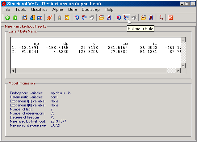
If you have opted for Cointegration Estimation in the "Cointegration Selection" frame on the Parameters tab on the Main Program window and you have selected a cointegration rank less than the number of endogenous variables and greater than zero on the Cointegration Rank Tests dialog, the second step in the estimation process is the selection of whether or not to estimate the model under linear restrictions on the cointegration vectors (β) and on the weights (α) on the cointegration relations.. This is performed on the Restrictions on (alpha,beta) dialog. Apart from selecting the restrictions to use for these parameters, a range of functions are available from the 7 Menus (File, Tools, Graphics, Alpha, Beta, Bootstrap, and Help) and the toolbar. The toolbar contains some of the most useful functions from the menus. Many of the functions on these menus can also be found on the previous dialog, i.e., on the Cointegration Rank Tests dialog. It should be kept in mind that these function take into account any restrictions you've decided that the model should satisfy.
|
Figure: The Restrictions on (alpha,beta) dialog in SVAR. |
The main purpose of this dialog is the selection of identifying and potentially over-identifying restrictions on the cointegration vectors. The cointegration space is, of course, already generically identified in the sense that it can be numerically uniquely determined (see, Johansen, 1995). The restrictions on β, the cointegration vectors that SVAR allows for can be expressed as follows:
βi = Hi*ψi, i=1,...,r,
where r is the cointegration rank, i.e., the number of cointegration vectors. The matrix Hi is here an (n+q1+d1)xs matrix, where n is the number of endogenous variables, q1 is the number of exogenous I(1) variables, and d1 is equal to 1 if the model has either a constant or a linear trend that has been restricted to the cointegration space. Otherwise the d1 parameter is 0. The s parameter depends on the number of restrictions that you would like to impose on β. βi is here an (n+q1+d1)x1 vector, while ψi is an sx1 vector. The parameter s is at most equal to n+q1+d1+1-r and at least equal to 1. In the former case, βi is (potentially) exactly identified and in the latter case known with certainty once a normalizing variable has been selected. The choice of normalizing variable determines which parameter is set to unity.
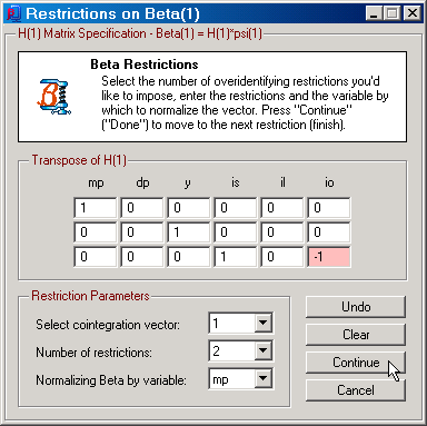
SVAR makes every attempt to facilitate the selection of Hi. The Figure below presents a case with 6 endogenous variables when the cointegration rank has been set to 2. The model here includes real money (mp), inflation (dp), real income (y), a short-term interest rate (is), a long-term interest rate (il), and the own rate of return on money (io). To identify a long-run money demand relation for this system with a unit parameter on real money, zero parameters on inflation and the long-term interest rate, a free parameter on real income and a free parameter on the opportunity cost variable (is-io), the number of over-identifying restrictions is 2, while H(1) is a 6x3 matrix as shown below. Notice that SVAR writes the transpose of the Hi matrix on screen. Also, changes to the individual elements is marked by a pinkish background color. Clicking on the Undo button resets the dialog to the initial state, while clicking on the Clear button resets the dialog to its default status.
SVAR handles the determination of the s parameter internally. What the user has to select is the number of over-identifying restrictions to impose on each cointegration vector. The dimension of the Hi matrix will automatically change as you change the value on the Number of Restrictions drop-down menu in the Figure below.
|
Figure: Specifying the restrictions on the first cointegration vector. |
The issue of whether or not the selected Hi matrices and normalizing variables prove to be identifying is tested by SVAR once you start estimation of β under the restrictions. If the restrictions do not satisfy the identification test, SVAR will inform you about this and abort estimation to allow you to change you Hi and normalizing variable choices. See also Cointegration Space section under the Identification heading.
Estimation of the model under the restrictions on β is performed using the switching algorithm described in Johansen (1995). See also Johansen (1996), section 7.2.3. Given that the model involves over-identifying restrictions, an LR-test is calculated. The results are presented on the Restrictions on Beta dialog, where you can also make further analysis of the restricted β model before you decide whether or not to use the restrictions in the forthcoming analysis of the cointegrated VAR system.
Once you have imposed a set of (over-)identifying restrictions on the cointegration vectors, it is possible to analyse the cointegrated VAR model with linear restrictions on the weights (α) on the cointegration relations. Theoretically, it is possible to also consider restrictions on α without first have identified β in an economic sense. However, SVAR does not allow for this since "good modelling practise" strongly suggests that economic identification of β should be pursued before attempting to analyse α. One may, of course, regard α as not having much meaningful interpretation however one has identified β, but this line of argumentation will be ignored here!
Linear restrictions on α can be studied in SVAR. To set up a set of restrictions, click on the "Restrict alpha" button on the Toolbar or on the "Restrict Alpha" option on the Alpha Menu. This opens a dialog, such as the one displayed in the Figure below.
|
Figure: Specifying the restrictions on the α matrix. |
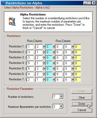
To specify a set of linear restrictions you can first choose the number of restrictions and the maximum number of parameters per restriction. This first should be rather obvious while the second selection makes it possible to involve more than one parameter in a given restrictions. You then proceed by selecting the individual α elements though their row and column index, the constant each such parameter should be multiplied by, and what the sum of these terms should add up to. The first element in such a linear combination of parameters is always multiplied by unity.
Estimation of the cointegrated VAR subject to α (and β) restrictions is carried out in one of two ways. If you have check marked the option "Re-estimate beta when estimating alpha, C or B under restrictions" on the Cointegration tab on the Preferences dialog, a switching algorithm will be employed, where all parameters but β are first estimated conditional on the estimated β matrix based on its restrictions (and where the rest of the parameters were unrestricted). Given these new parameter values that satisfy your α restrictions, β is re-estimated conditional on these values yielding potentially a new estimate of β. These steps are then re-iterated until the convergence criterion is met. This criterion is, for instance, given by the maximum absolute value of the gradient vector for all parameters given that you have check marked the option "Use gradient for restricted beta convergence" on the Cointegration tab on the Preferences dialog. SVAR will otherwise use the maximum absolute parameter change for β as its criterion. Once the algorithm has converged, LR-tests of the null hypotheses are calculated and the results are presented on the Restrictions on Alpha dialog. There you can make further analysis of the estimated cointegrated VAR satisfying both the α and β restrictions.
If you have not check marked the option "Re-estimate beta when estimating alpha, C or B under restrictions" on the Cointegration tab on the Preferences dialog, the original restricted estimates of β are kept and only the initial step of estimating all the other parameters subject to the α restrictions conditional on β is performed. Asymptotically, it won't matter which approach is used, but it may matter a lot in small samples.
| • | View Data: Allows you to view data in a file format that SVAR can read (see Data Input for details). |
| • | Save Cointegration Relations: Allows you to save the estimated cointegration relations in a text file. |
| • | Save Transitory Components: Allows you to save the transitory components (determined by a Beveridge-Nelson decomposition) in a text file. This feature requires that the model has at least one unit root. |
| • | Save Residuals: Allows you to save the estimated residuals in a text file. |
| • | Center Window: Centers the dialog window. |
| • | Return: Takes you back to the Cointegration Rank Tests window and resets the cointegration rank to the original full rank selection without any over-identifying or normalizing restrictions on β and no restrictions on α. Available on the Toolbar. |
| • | Continue: If you've selected to estimate a reduced form model on the Parameters tab of the main program window, then this will end the empirical analysis. If you've instead opted for a structural form, then this will take you to the Identification & Estimation dialog. Available on the Toolbar. |
| • | Quit: If you've selected to estimate a structural form of the cointegrated VAR, then this will end the empirical analysis. If not, then this function is handled by the Continue function instead. Available on the Toolbar. |
| • | Serial Correlation: See the Tools Menu on the Cointegration Rank Tests dialog. |
| • | ARCH: See the Tools Menu on the Cointegration Rank Tests dialog. |
| • | Normality: See the Tools Menu on the Cointegration Rank Tests dialog. |
| • | Parameter Constancy: See the Tools Menu on the Cointegration Rank Tests dialog. |
| • | Lag Order: See the Tools Menu on the Cointegration Rank Tests dialog. |
| • | Weak Exogeneity: See the Tools Menu on the Cointegration Rank Tests dialog. |
| • | Granger Causality: See the Tools Menu on the Cointegration Rank Tests dialog. |
| • | Multi-Step Granger Causality: See the Tools Menu on the Cointegration Rank Tests dialog. |
| • | Exclusion è |
| • | First Differences: See the Tools Menu on the Cointegration Rank Tests dialog. |
| • | Cointegration Space è |
| • | Exclusion: See the Tools Menu on the Cointegration Rank Tests dialog. |
| • | Stationarity: See the Tools Menu on the Cointegration Rank Tests dialog. |
| • | Common Cycles: See the Tools Menu on the Cointegration Rank Tests dialog. |
| • | Deterministic Variables è |
| • | Exclusion: See the Tools Menu on the Cointegration Rank Tests dialog. |
| • | Long Run: See the Tools Menu on the Cointegration Rank Tests dialog. |
| • | Proportionality: See the Tools Menu on the Cointegration Rank Tests dialog. |
| • | C-Matrix: See the Tools Menu on the Cointegration Rank Tests dialog. |
| • | Long Run GIRs: See the Tools Menu on the Cointegration Rank Tests dialog. |
| • | Residual Analysis: See the Tools Menu on the Cointegration Rank Tests dialog. |
| • | Short Run Dynamics: See the Tools Menu on the Cointegration Rank Tests dialog. |
| • | Distribution: See the Tools Menu on the Cointegration Rank Tests dialog. |
| • | Cointegration Relations: See the Graphics Menu on the Cointegration Rank Tests dialog. Available on the Toolbar. |
| • | Permanent and Transitory Components: See the Graphics Menu on the Cointegration Rank Tests dialog. Available on the Toolbar. |
| • | Residuals: See the Graphics Menu on the Cointegration Rank Tests dialog. Available on the Toolbar. |
| • | Fitted Terms: See the Graphics Menu on the Cointegration Rank Tests dialog. |
| • | Forecasting: See the Graphics Menu on the Cointegration Rank Tests dialog. Available on the Toolbar. |
| • | Forecast Variable Transformations: See the Graphics Menu on the Cointegration Rank Tests dialog. |
| • | Recursive Chow Test: See the Graphics Menu on the Cointegration Rank Tests dialog. Available on the Toolbar. |
| • | Recursive Fluctuation Test: See the Graphics Menu on the Cointegration Rank Tests dialog. Available on the Toolbar. |
| • | Generalized Impulse Responses: See the Graphics Menu on the Cointegration Rank Tests dialog. |
| • | Dummy Impulse Responses: See the Graphics Menu on the Cointegration Rank Tests dialog. |
| • | Log-likelihood and Beta: This function is enabled once the cointegration vectors have been properly identified; see discussion above on restrictions on beta. The log-likelihood and beta function allows you to provide plots of the log-likelihood function relative to one or two β parameters. The shape of the log-likelihood function can either be for fixed values of all the other parameters, or these can be re-estimated for each value of the β parameters of interest. The latter parameters take on values from a grid that you can select from the Log-likelihood and Beta dialog; see Figure below. |
|
Figure: The log-likelihood and beta selection dialog. |
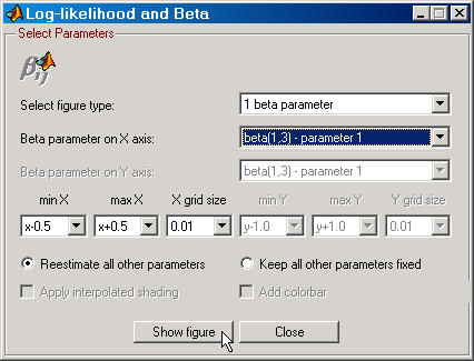
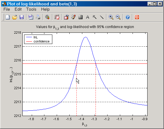
This function provides one way to approximate unconditional x percent confidence bands for the estimated free parameters of the cointegration vectors. The x parameter here is determined from your selection of confidence band size on the Parameters tab on the main program window. In the Figure above, the log-likelihood will be plotted against 1 beta parameter, given by β1,3, i.e., the third element of the first cointegration vector. The grid is constructed with the maximum likelihood element in the center and with minimum and maximum values that can be chosen the set of predefined values relative to the center value. The distance between two β1,3 values is given by the X grid size parameter above. The selection to "Re-estimate of other parameters* guarantees that the largest possible value of the likelihood is obtained given the restrictions the model should satisfy. For each fixed β1,3 value in full grid, all remaining free parameters of the model are re-estimated and the value of the log-likelihood is calculated. When β1,3 is equal to the center value (the maximum likelihood estimate), the log-likelihood function takes on its largest possible value. This gives us a range of β1,3 values and the log-likelihood value thus linked to each one of them. To determine a confidence band, an x percent value of the log-likelihood function is determined from the definition of the LR statistic, the observed largest value of the log-likelihood function, and the critical value from the chi-square distribution with 1 degree of freedom that corresponds to x percent. In case x=95, the critical value is 3.84, and so on. This means that the value of the log-likelihood function that yields exactly 3.84 is given by:
lnL(95 percent crit) = lnL(max)-[3.84/2].
We can now compare the value of the log-likelihood when the LR-test is equal to 3.84 to the values of the log-likelihood function for the different β1,3 graphically and determine the 95 percent upper and lower bounds from these given that a sufficiently large grid has been selected. This is illustrated in the Figure below.
|
Figure: Plot of the log-likelihood function for given values of β1,3 along with the log-likelihood value that provides an LR(1) statistic equal to 3.84, and the minimum and maximum values of β1,3 that yield these log-likelihood values. |
| • | Eigenvalues of Companion Matrix: See the Graphics Menu on the Cointegration Rank Tests dialog. |
| • | Restrict Alpha: Opens the dialog for setting up restrictions on the weights on the cointegration relations; see Figure above. Available on the Toolbar. |
| • | Estimate Alpha: Starts the estimation of the cointegrated VAR subject to the (over-)identifying restrictions on α and β that you have selected. Once the estimation procedure has completed its mission, the Restrictions on Alpha dialog is displayed with the results. Available on the Toolbar. |
| • | Unrestrict Alpha: This function is enabled once you have chosen to use a restricted α estimate. If you want the model to once again be based on the unrestricted α estimate (but keeping the possibly over-identified β estimate), you should run this function. Available on the Toolbar. |
| • | Open Alpha Restrictions: Opens a dialog for selecting α restrictions that have been saved to file. All restrictions created through the Restrict Alpha function are saved into restriction files. These are internally named "G-nxr-modelname.rest", where n is the number of endogenous variables and r the number of cointegration relations. The "modelname" refers to the name of the model as shown on the main program window, e.g., "money-real-euro1112-sa-9-9-2002-wk1" in the Figure on the main program window page. Available on the Toolbar. |
| • | Save Alpha Restrictions: Opens a dialog from where you can save α restriction files under a different name for, e.g., later use. Available on the Toolbar. |
| • | Restrict Beta: Opens the dialog for setting up restrictions on the cointegration vectors; see Figure above. Available on the Toolbar. |
| • | Estimate Beta: Starts the estimation of the cointegrated VAR subject to the (over-)identifying restrictions on β that you have selected provided that the selected restriction are identifying. Once the estimation procedure has completed its mission, the Restrictions on Beta dialog is displayed with the results. Available on the Toolbar. |
| • | Unrestrict Beta: This function is enabled once you have chosen to use the new beta from the Restrictions on Beta dialog and returned to the current dialog. In case you've changed your mind about the selected cointegration vectors for the empirical model, this function allows you to reset the selected cointegration vectors to the original unrestricted vectors that were provided on the Cointegration Rank Tests dialog. Available on the Toolbar. |
| • | Open Beta Restrictions: Opens a dialog for selecting β restrictions that have been saved to file. All restrictions created through the Restrict Beta function are saved into restriction files. These are internally named "H_i_nxrxd1+q1-modelname.rest", where i refers to βi, n is the number of endogenous variables, r the number of cointegration relations, d1 the number of deterministic variables restricted to the cointegration relations (1 or 0), while q1 is the number of exogenous I(1) variables. The "modelname" refers to the name of the model as shown on the main program window, e.g., "money-real-euro1112-sa-9-9-2002-wk1" in the Figure on the main program window page. Available on the Toolbar. |
| • | Save Beta Restrictions: Opens a dialog from where you can save β restriction files under a different name for, e.g., later use. Available on the Toolbar. |
| • | Estimate Beta (or Alpha, Beta) Recursively: Runs recursive estimation of the free β parameters, along with the LR test of any over-identifying restrictions, the Nyblom test for the constancy of the cointegration space (if the option "Compute Nyblom test for beta under beta restrictions" is check marked on the Recursion tab on the Preferences dialog), and the maximum non-unit eigenvalue of the companion matrix (if the option "Enable recursive estimation of companion matrix's max eigenvalue" is check marked on the Recursion tab on the Preferences dialog). In addition, if the option "Enable recursive estimation of alpha" is check marked on the Recursion tab on the Preferences dialog, the function will also provide graphs of recursively estimated α parameters, along with LR-tests of α restrictions, given that the model should satisfy such restrictions. Available on the Toolbar. |
| • | Alpha, Delta, Gamma: Opens the dialog for bootstrapping the α, δ, Γ parameters, and any tests of restrictions on α. See Bootstrapping the Alpha, Delta, Gamma parameters for details. |
| • | Beta: Open the dialog for bootstrapping the free β parameters and, if the cointegration vectors are over-identified, the LR-test of these restrictions. See Bootstrapping the Beta parameters for details. |
| • | Nyblom Distribution: See the Bootstrap submenu on the Simulation menu on the Cointegration Rank Tests dialog. |
| • | Recursive Fluctuation Test: See the Bootstrap submenu on the Simulation menu on the Cointegration Rank Tests dialog. |
| • | Specification Tests: See the Bootstrap submenu on the Simulation menu on the Cointegration Rank Tests dialog. |
| • | Markov Switching Test: See the Bootstrap submenu on the Simulation menu on the Cointegration Rank Tests dialog. |
| • | Restrictions on alpha,beta: Opens the help file on this page. |
| • | Common Cycles - PDF File: Given that SVAR knows this file exists and where a PDF viewer is located on your hard drive, the PDF documentation on common cycles can be opened directly from this menu item. |
| • | Generalized Impulse Responses - PDF File: Given that SVAR knows this file exists and where a PDF viewer is located on your hard drive, the PDF documentation on generalized impulse responses can be opened directly from this menu item. |