


If you have opted for Structural Form in the "Model Type Selection" frame on the Parameters tab of the Main Program window, the structural form analysis as well as the analysis of reduced form long-run restrictions (restrictions on C) is carried out through the Identification & Estimation dialog. SVAR currently supports three types of identification of shocks in its classical analysis. They are:
| 1. | Contemporaneous restrictions; |
| 2. | Long-run restrictions; |
| 3. | A combination of the above. |
You can set the default choice of these three on the Estimation tab on the Preferences dialog. This default choice is determined by the Default identification specification. Since identifying restrictions are stored in *.rest files on your hard disk, the first time you reach the Identification & Estimation dialog, the Restrictions Selection frame options will all be disabled and with the "Contemporaneous restrictions" radio button selected. Once valid identification restrictions files exist, the "Default identification" choice will be obeyed. Technical aspects of identification will not be discussed below, but are instead considered in the Identification section of this help file. The Identification & Estimation dialog is displayed in the Figure below.
|
Figure: The Identification & Estimation dialog in SVAR. |
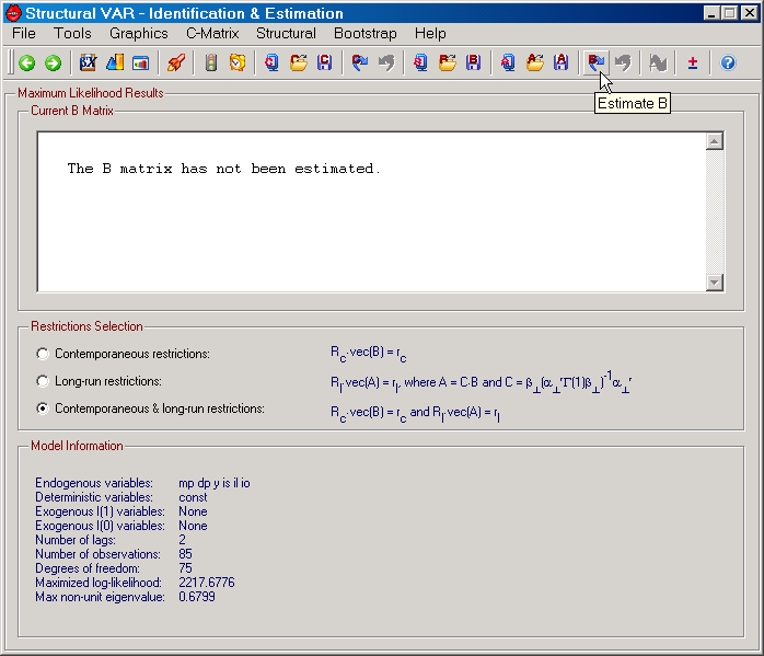
Apart from setting up the appropriate identifying restrictions for your structural model, a wide range of tools are available on the 7 menus (File, Tools, Graphics, C-Matrix, Structural, Bootstrap, and Help) and on the toolbar of the Identification & Estimation dialog. The toolbar contains some of the most useful functions from the menus.
In order to achieve exact identification of a structural (cointegrated) VAR model with n variables, n*n restrictions are required. Further restrictions can also be considered and in that case the extra over-identifying restrictions can be tested just like any other over-identifying restrictions on the model.
SVAR always imposes n*(n+1)/2 restrictions by using the assumption that the covariance matrix of the structural shocks is the identity. Exact identification therefore requires an additional n*(n-1)/2 restrictions. Unless the cointegration rank is equal to the number of endogenous variables, at least some of the restrictions have to be imposed on the contemporaneous effects of the shocks. These effects are represented by the nxn matrix B is SVAR. In the Figure above it can be seen that the restrictions on B have to be linear, but that they may involve cross-equation restrictions.
|
Figure: The contemporaneous identifying restrictions dialog. |
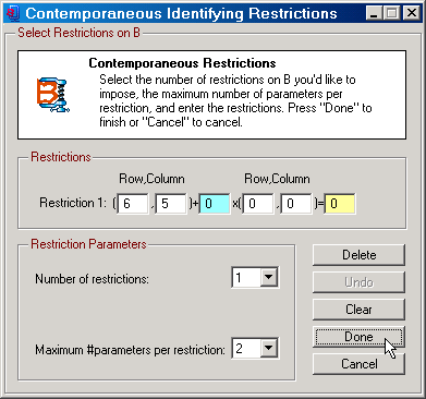
In the Figure above it can be seen that the model involves 1 contemporaneous identifying restriction, namely that B(6,5) = 0. The example model here has n=6 and therefore also 6 structural shocks. The above restriction implies that the 5th shock has a zero contemporaneous effect on the 6th endogenous variable. This is not sufficient for exact identification since (in addition to the 21 restrictions on the covariance matrix of the structural shocks) this would require 15 restrictions on the parameters. The remaining 14+ any over-identifying restrictions will have to be handled through long-run restrictions.
Long-run restrictions are given as linear restrictions on the matrix A, the long-run total impact matrix. This matrix is given by the product of the matrix C and the matrix B. The C matrix is simply the reduced long-run impact matrix and in the case of cointegration restrictions is determined by the parameters of the cointegrated VAR model, as displayed in the top Figure on this page. The B matrix is, as already discussed, the parameters measuring the contemporaneous affects of the shocks.
|
Figure: The long-run identifying restrictions dialog. |
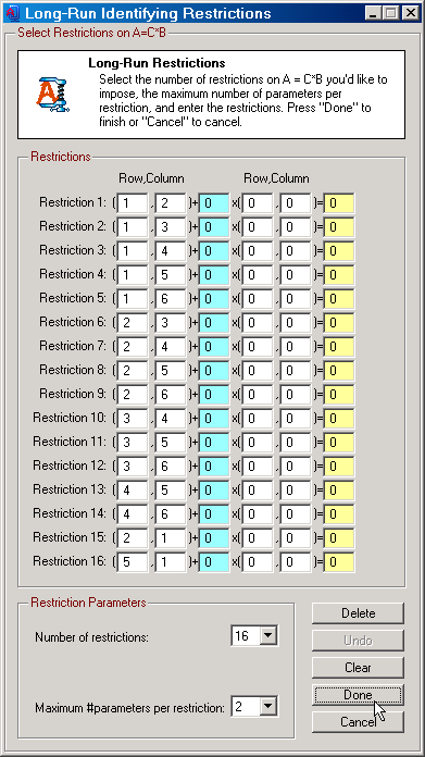
In the Figure above, a total of 16 restrictions have been imposed on the A matrix. In combination with the 1 restriction on B, this means that at total of 17 identifying restrictions are considered. Since n=6, this means that there are 2 over-identifying restrictions. These restrictions can be represented by A(2,1) = A(5,1) = 0, although other alternatives in the dialog above can serve this purpose as well.
The model here has r=2 cointegration relations. This means that both the C and the A matrix has rank k=n-r=4. The structure of the long-run restrictions here implies that 4 additional elements of A are zero. Specifically,
A(5,5) = A(5,6) = A(6,5) = A(6,6) = 0.
This follows immediately from the rank requirement for the A matrix. See the Common Trends Model - Part 1 and Part 2 for additional discussions on this issue.
Once all identification restrictions have been chosen you can attempt to estimate the structural model by clicking on the Estimate B button on the toolbar. When this function is run it first performs a test for local identification and returns an error message in case the restrictions are deemed non-identifying. If they check out OK, estimation commences.
Since
A = C*B
it follows that linear restrictions on A generally translate into non-linear restrictions on the parameters of the structural cointegrated VAR model. SVAR supports two approaches to this estimation related problem.
Vlaar (2004) suggested to treat the reduced form estimate of C as given. This means that all identifying restrictions are imposed on the B matrix. As long as the structural model does not involve any over-identifying restrictions this assumption does not matter. The reason is that all exactly identified models are observationally equivalent and, hence, only care must be taken to ensure that asymptotic inference based on the estimated structural parameters take into account that C is estimated. The Vlaar procedure takes care of this. See the Method option on the Estimation tab on the Preferences dialog.
An discussed on the An Over-Identification Issue page, there are over-identifying restrictions that the Vlaar approach cannot deal with. SVAR provides two solutions to this problem. The first is to allow for linear restrictions on C (available from the C-Matrix menu and from the toolbar), while the second is not to treat the reduced form estimate of C as given. More generally, when the model involves over-identifying restrictions, the assumption that the estimate of C is treated as given, means that the estimated structural parameters are not ML estimates. Hence, the second approach is typically preferred in these situations.
SVAR applies the Vlaar approach if estimation of the reduced form parameters is separated from estimation of B on the Method option on the Estimation tab on the Preferences dialog. This is the first option among 3 possible. The second option attempts to estimate the reduced form parameters and B jointly, while the third uses Bayesian analysis. Currently, the second classical method is not full information maximum likelihood when the model involves long-run restrictions and some of the restrictions are over-identifying. This statement is true even when β is estimated jointly with the reduced form. Instead, SVAR examines the restrictions to constructs a range of sets containing one set of exactly identifying restrictions and another set of the over-identifying restrictions. The total number of such sets depends on the number of restrictions and the number of over-identifying restrictions. For all such sets which are feasible (called cases by SVAR) the exactly identifying restrictions are imposed on B, while the over-identifying restrictions are either imposed on C or on B. Among all feasible sets, the set of restrictions that yields the largest likelihood value is chosen. This approach is clearly not maximum likelihood since none of the over-identifying restrictions are imposed jointly on C and on B. At the same time, the approach is generally superior to the Vlaar approach since the latter only imposes over-identifying restrictions on B. Finally, it should be noted that this second method is likely to be changed into a full information maximum likelihood procedure at some stage in the future.
| • | View Data: Allows you to view data in a file format that SVAR can read (see Data Input for details). |
| • | Save Cointegration Relations: Allows you to save the estimated cointegration relations in a text file. |
| • | Save Transitory Components: Allows you to save the transitory components (determined by a Beveridge-Nelson decomposition) in a text file. This feature requires that the model has at least one unit root. |
| • | Save Residuals: Allows you to save the estimated residuals in a text file. |
| • | Center Window: Centers the dialog window. |
| • | Return: Takes you back to either the Restrictions on (alpha,beta) dialog (if the cointegration rank is between 1 and n-1) or the Cointegration Rank Tests dialog (if the cointegration rank is 0 or 1). In the latter case, all parameters are reset to their original values for the unrestricted model, while in the former case they are reset to the values for the selected rank but where the model is otherwise unrestricted. Available on the Toolbar. |
| • | Done: Ends the estimation. Available on the Toolbar. |
| • | Serial Correlation: See the Tools Menu on the Cointegration Rank Tests dialog. |
| • | ARCH: See the Tools Menu on the Cointegration Rank Tests dialog. |
| • | Normality: See the Tools Menu on the Cointegration Rank Tests dialog. |
| • | Parameter Constancy: See the Tools Menu on the Cointegration Rank Tests dialog. |
| • | Lag Order: See the Tools Menu on the Cointegration Rank Tests dialog. |
| • | Weak Exogeneity: See the Tools Menu on the Cointegration Rank Tests dialog. |
| • | Granger Causality: See the Tools Menu on the Cointegration Rank Tests dialog. |
| • | Multi-Step Granger Causality: See the Tools Menu on the Cointegration Rank Tests dialog. |
| • | Exclusion è |
| • | First Differences: See the Tools Menu on the Cointegration Rank Tests dialog. |
| • | Cointegration Vectors: Displays the estimated cointegration vectors along with estimated asymptotic conditional standard errors when these are available. |
| • | Common Cycles: See the Tools Menu on the Cointegration Rank Tests dialog. |
| • | Deterministic Variables è |
| • | Exclusion: See the Tools Menu on the Cointegration Rank Tests dialog. |
| • | Long Run: See the Tools Menu on the Cointegration Rank Tests dialog. |
| • | Proportionality: See the Tools Menu on the Cointegration Rank Tests dialog. |
| • | A-matrix: Displays the estimated A matrix along with its estimated asymptotic standard errors for the structural model. |
| • | B-matrix: Displays the estimated B matrix along with its estimated asymptotic standard errors for the structural model. |
| • | C-Matrix: See the Tools Menu on the Cointegration Rank Tests dialog. |
| • | Long Run GIRs: See the Tools Menu on the Cointegration Rank Tests dialog. |
| • | Residual Analysis: See the Tools Menu on the Cointegration Rank Tests dialog. |
| • | Short Run Dynamics: See the Tools Menu on the Cointegration Rank Tests dialog. |
| • | Variance Decompositions: Displays the estimated forecast error variance decompositions for the levels of the endogenous variables of the structural model along with estimated asymptotic standard errors up to the Number of Responses horizon selected on the Parameters tab on the Main Program window. |
| • | Distribution: See the Tools Menu on the Cointegration Rank Tests dialog. |
| • | Cointegration Relations: See the Graphics Menu on the Cointegration Rank Tests dialog. Available on the Toolbar. |
| • | Permanent and Transitory Components: See the Graphics Menu on the Cointegration Rank Tests dialog. Available on the Toolbar. |
| • | Permanent and Transitory Shock Components: Once the structural model has been estimated, it is possible to calculate the contributions to the Beveridge-Nelson type permanent and transitory components decomposition that is due to the various structural shocks. This function performs this type of decomposition. |
| • | Residuals: See the Graphics Menu on the Cointegration Rank Tests dialog. Available on the Toolbar. |
| • | Fitted Terms: See the Graphics Menu on the Cointegration Rank Tests dialog. |
| • | Forecasting: See the Graphics Menu on the Cointegration Rank Tests dialog. Available on the Toolbar. |
| • | Forecast Variable Transformations: See the Graphics Menu on the Cointegration Rank Tests dialog. |
| • | Recursive Chow Test: See the Graphics Menu on the Cointegration Rank Tests dialog. Available on the Toolbar. |
| • | Recursive Fluctuation Test: See the Graphics Menu on the Cointegration Rank Tests dialog. Available on the Toolbar. |
| • | Impulse Responses: Displays impulse responses for the levels of the endogenous variables of the structural model along with X percent confidence bands. X is given by the Confidence Band Size selection and the number of responses by the Number of Responses horizon selected on the Parameters tab on the Main Program window. Available on the Toolbar. |
| • | Historical Decompositions: For a given forecast horizon, historical decompositions of the forecasts errors are graphed for each selected variable. A decomposition is performed for each structural shock. The forecast horizon can be selected between 1 period and P periods, where P is equal to 5 years, i.e. P=20 for quarterly data. The default value is taken from the "Default forecast horizon" option on the Forecasting tab on the Preferences dialog. |
| • | Generalized Impulse Responses: See the Graphics Menu on the Cointegration Rank Tests dialog. |
| • | Dummy Impulse Responses: See the Graphics Menu on the Cointegration Rank Tests dialog. |
| • | Log-likelihood and Beta: See the Graphics Menu on the Restrictions on (alpha,beta) dialog. |
| • | Eigenvalues of Companion Matrix: See the Graphics Menu on the Cointegration Rank Tests dialog. |
| • | C-Restrictions: Opens the dialog for setting up restrictions on the C matrix. Available on the Toolbar. |
| • | Open C Restrictions: Opens a dialog for selecting C restrictions that have been saved to file. All restrictions created through the C-Restriction function are saved into restriction files. These are internally named "C-nxr-modelname.rest", where n is the number of endogenous variables and r the number of cointegration relations. The "modelname" refers to the name of the model as shown on the main program window, e.g., "money-real-euro1112-sa-9-9-2002-wk1" in the Figure on the main program window page. Available on the Toolbar. |
| • | Save C Restrictions: Opens a dialog from where you can save C restriction files under a different name for, e.g., later use. Available on the Toolbar. |
| • | Estimate C: Starts the estimation of the cointegrated VAR subject to the restrictions on C that you have selected. Once the estimation procedure has completed its mission, the Restrictions on C dialog is displayed with the results. Available on the Toolbar. |
| • | Undo C: This function is enabled once you have chosen to use the new C from the Restrictions on C dialog and returned to the current dialog. In case you've changed your mind about the selected C restrictions for the empirical model, this function allows you to reset the model parameters to those estimated prior to the C restrictions estimation. Available on the Toolbar. |
| • | Contemporaneous Restrictions: Opens the dialog for setting up linear restrictions on B, i.e., on the contemporaneous effect of the shocks; see Figure above. Available on the Toolbar. |
| • | Open Contemporaneous Restrictions: Opens a dialog for selecting contemporaneous restrictions that have been saved to file. All restrictions created through the Contemporaneous Restrictions function are saved into restriction files. These are internally named "F-nxr-modelname.rest", where n is the number of endogenous variables and r the number of cointegration relations. The "modelname" refers to the name of the model as shown on the main program window, e.g., "money-real-euro1112-sa-9-9-2002-wk1" in the Figure on the main program window page. Available on the Toolbar. |
| • | Save Contemporaneous Restrictions: Opens a dialog from where you can save contemporaneous restriction files under a different name for, e.g., later use. Available on the Toolbar. |
| • | Long-Run Restrictions: Opens the dialog for setting up linear restrictions on A, i.e., on the long-run effect of the shocks; see Figure above. Available on the Toolbar. |
| • | Open Long-Run Restrictions: Opens a dialog for selecting long-run restrictions that have been saved to file. All restrictions created through the Long-Run Restrictions function are saved into restriction files. These are internally named "LF-nxr-modelname.rest", where n is the number of endogenous variables and r the number of cointegration relations. The "modelname" refers to the name of the model as shown on the main program window, e.g., "money-real-euro1112-sa-9-9-2002-wk1" in the Figure on the main program window page. Available on the Toolbar. |
| • | Save Long-Run Restrictions: Opens a dialog from where you can save long-run restriction files under a different name for, e.g., later use. Available on the Toolbar. |
| • | Sign Shocks: The shocks of a Structural VAR model can only be uniquely determined up to its sign, i.e., B*ηt = (B*H)*(H-1*ηt), where ηt is the original vector of structural shocks and H is a diagonal matrix with diagonal entries 1 or -1. This function allows you to make sure that each shock has a well defined positive or negative contemporaneous effect on one of the endogenous variables. This function will first test if the identifying restrictions you have chosen are locally identifying. If the test comes out in favor of identification, the Signs of Structural Shocks dialog is opened. |
|
Figure: The dialog for selecting contemporaneous shock signs. |
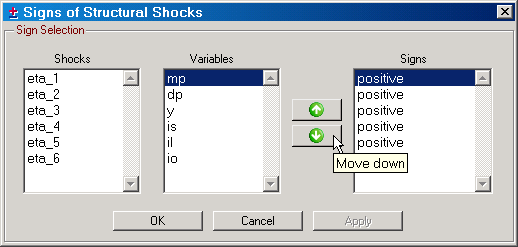
By default, SVAR does not impose any particular sign on the effect of shocks. Once signs have been selected, they are stored in on your hard drive under the name "signs-nxr-modelname.rest", where n is the number of endogenous variables and r is the number of cointegration relations. The "modelname" refers to the name of the model as shown on the main program window, e.g., "money-real-euro1112-sa-9-9-2002-wk1" in the Figure on the main program window page. Once created, these sign "restrictions" files can only be deleted manually. Available on the Toolbar.
| • | Estimate B: Starts the estimation of the parameters of the structural VAR model once the restrictions have passed the local identification test. Once the estimation procedure has completed its task, the Restrictions on B and A=C*B dialog is displayed with the results. Available on the Toolbar. |
| • | Undo B: This function is enabled once you have chosen to use the new B matrix from the Restrictions on B and A=C*B dialog. In case you've changed your mind about the selected identifying restrictions for the empirical model, this function allows you to reset the model parameters to those prior to the B restrictions estimation. Available on the Toolbar. |
| • | Alpha, Delta, Gamma: Opens the dialog for bootstrapping the α, δ, Γ parameters, and any tests of restrictions on α. See Bootstrapping the Alpha, Delta, Gamma parameters for details. |
| • | Beta: Open the dialog for bootstrapping the free β parameters and, if the cointegration vectors are over-identified, the LR-test of these restrictions. See Bootstrapping the Beta parameters for details. |
| • | Nyblom Distribution: See the Bootstrap submenu on the Simulation menu on the Cointegration Rank Tests dialog. |
| • | Structural Parameters: Opens the dialog for bootstrapping the A and B parameters along with the impulse responses and the LR-test of over-identifying restrictions. See Bootstrapping the Structural Parameters for details. |
| • | Recursive Fluctuation Test: See the Bootstrap submenu on the Simulation menu on the Cointegration Rank Tests dialog. |
| • | Specification Tests: See the Bootstrap submenu on the Simulation menu on the Cointegration Rank Tests dialog. |
| • | Help Topics: Opens the help file on the Identification page. Available on the Toolbar. |
| • | Identification and Estimation: Opens the help file on this page. |
| • | Common Cycles - PDF File: Given that SVAR knows this file exists and where a PDF viewer is located on your hard drive, the PDF documentation on common cycles can be opened directly from this menu item. |
| • | Estimate C - PDF File: Given that SVAR knows this file exists and where a PDF viewer is located on your hard drive, the PDF documentation on estimation of the C matrix under linear restrictions can be opened directly from this menu item. This file can also be downloaded from: http://www.texlips.net/download/estimate-c.pdf. |
| • | Generalized Impulse Responses - PDF File: Given that SVAR knows this file exists and where a PDF viewer is located on your hard drive, the PDF documentation on generalized impulse responses can be opened directly from this menu item. |
| • | Variance Decompositions - PDF File: Given that SVAR knows this file exists and where a PDF viewer is located on your hard drive, the PDF documentation on asymptotic distribution of forecast error variance decompositions can be opened directly from this menu item. This file can also be downloaded from: http://www.texlips.net/download/var-decomp.pdf. |