If you have opted for Cointegration Estimation in the "Cointegration Selection" frame on the Parameters tab on the Main Program window, the first step in the estimation process is the selection of the cointegration rank for your model. This is performed on the Cointegration Rank Tests dialog. Apart from selecting the proper rank, a range of functions are available from the 5 Menus (File, Tools, Graphics, Simulation, and Help) and the toolbar. The toolbar contains some of the most useful functions from the menus. Below the functions on the 5 menus will be briefly discussed below.
|
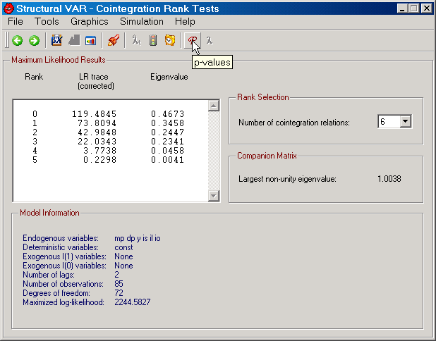
Figure: The cointegration rank tests dialog in SVAR.
|
The main purpose on this dialog is to select the cointegration rank. The currently selected rank is presented in the Rank Selection frame (see Figure above) and you can change it by using the drop-down menu. Integer values between 0 and the number of endogenous variables can be chosen.
As one aid for this selection the cointegration rank tests, represented by the LR (Likelihood Ratio) Trace tests, are presented in the upper left corner of the Maximum Likelihood Results frame. If SVAR has sufficient information about the asymptotic distribution for these tests, the toolbar will contain either a p-value button (as in the Figure above) or a critical value button as well as an eigenvalue button. The eigenvalues are the ones used to calculate the trace tests. On the Cointegration tab on the Preferences dialog the choice you've made about Trace test critical value or p-value determines which of the p-value and critical value buttons is displayed here. The p-values and the critical values are taken from a number of sources, including the Working Paper version of MacKinnon, Haug and Michelis, L. (1999), through simulation of the trace test using SVAR itself (see, e.g., Harbo, Johansen, Nielsen and Rahbek, 1998), and using the method suggested by Boswijk and Doornik (2005). Every attempt has been made to use the best possible source for the numerical quantile values of the asymptotic distribution of the trace test.
Other aids for the selection of the cointegration rank are also available. The perhaps most interesting and special tool is located on the Simulation menu, where you can open the Bootstrap Trace Distribution dialog.
The largest non-unit eigenvalue of the Companion matrix is presented below the Rank Selection frame. This value is determined by rewriting a VAR model with k lags into a VAR model with 1 lag by stacking vectors and using equivalence relations, the so called companion form. The eigenvalues of the matrix on the first lag in this representation are equal to the inverse of the roots to the lag polynomial for the original VAR model with k lags. The modulus of each such eigenvalue is computed and the largest non-unit value among these is presented in the Companion Matrix frame. Naturally, this value depends on how many cointegration relations you have chosen. Values below unity is expected for stationary processes.
At the bottom of the dialog, some general information about your model is given. Here you'll find the names of the variables, the number of lags and observations that are used, the number of free observations per equation (degrees of freedom), and the value of the maximized log-likelihood function. The latter value is computed from the Gaussian log-likelihood and it includes all constants from that function. Moreover, it depends on the cointegration rank you've selected.
File Menu
| • | View Data: Allows you to view data in a file format that SVAR can read (see Data Input for details). |
| • | Save Cointegration Relations: Allows you to save the estimated cointegration relations in a text file. |
| • | Save Transitory Components: Allows you to save the transitory components (determined by a Beveridge-Nelson decomposition) in a text file. This feature requires that the model has at least one unit root. |
| • | Save Residuals: Allows you to save the estimated residuals in a text file. |
| • | Center Window: Centers the dialog window. |
| • | Show p-values/Show Critical Values: For models where the asymptotic distribution of the trace test is known or has been simulated, SVAR can display p-values of critical values on the Cointegration Rank Tests dialog (see Figure above). Which one of these can be displayed depends on which option has been selected on the Cointegration tab on the Preferences dialog. When enabled, this menu item allows the user to switch from displaying the eigenvalues underlying the trace tests to the p-values or the critical values. Available on the Toolbar. |
| • | Show Eigenvalues: The reverse of the previous item. Allows the user to switch from displaying the p-values or the critical values of the trace tests to the underlying eigenvalues. Available on the Toolbar. |
| • | Return: Takes you back to the Main Program window and thus stops the estimation. Available on the Toolbar. |
| • | Continue: If you've selected a cointegration rank greater than 0 and the model contains at least one unit root, then this will take you to the Restrictions on (alpha,beta) dialog. Otherwise the empirical analysis will continue on the Identification and Estimation dialog (if you wish to analyse the model in Structural form - see Parameters tab on the Main Program window) or you're done! This function is also available on the toolbar, where you'll find a blue arrow pointing in the right direction. Available on the Toolbar. |
Tools Menu
| • | Serial Correlation: Allows you to view the results from two types of serial correlation tests. The first is a set of LM tests which tests if the residuals follow a VAR process under the alternative versus white noise under the null. The VAR process in the first case concerns only lag 1 of the residuals and in the second case lag q, with q=4 for quarterly data and q=12 for monthly. The test statistic is calculated as described in Johansen (1996), p. 22. The second type of serial correlation tests is the Ljung-Box Portmanteau statistic. This statistic is by default calculated as in Johansen (1996), p. 22, but can also be Bartlett corrected; see the "Correct Ljung-Box type Portmanteau statistic" option on the Statistics tab of the Preferences dialog.. |
| • | ARCH: The are the by now standard univariate LM tests for ARCH at lag 1 and at lag q, with q being the frequency of the data, i.e. q=4 for quarterly and so on. In addition, an LM test for multivariate ARCH of order 1 is calculated. This latter test either concerns all [n*(n+1)/2]^2 parameters on the first lag (default) or the n*(n+1)/2 diagonal elements of this matrix. The choice of multivariate ARCH model under the alternative can be selected on the Statistics tab on the Preferences dialog. |
| • | Normality: Four normality tests can be computed by SVAR. The first and second are the skewness and excess kurtosis Wald-type tests while the third is a Wald-type test of both these forms of non-normality; see Section 4.5.1 in Lütkepohl (1991) for details on the computation of λ(1), λ(2) and λ(3). The fourth test is the Omnibus test suggested by Doornik and Hansen (1994). This test is calculated exactly as described in their article. |
| • | Parameter Constancy: Four groups of parameter constancy tests may be computed. Three of these groups concern the parameters on deterministic and stationary variables, while one group concerns the cointegration space. The latter are the Nyblom tests suggested by Hansen and Johansen (1999), where the version suggested by Bruggeman, Donati and Warne (2003) are used by default. Of the remaining three groups, the first are based on the so called LSTR1 model of Teräsvirta (1998). The tests are calculated both in their LM version and in their F version using a first and a third order Taylor expansion. The tests are calculated equation-by-equation and for the different groups of parameters in the model, i.e., parameters on deterministic variables, lagged first differences, and parameters on cointegration relations. The second group of parameter constancy tests for parameters on deterministic and stationary variables are the Chow inspired tests. These concerns the 1-step ahead on an equation-by equation basis, and the Chow break-point and sample-split tests on a system basis (see Candelon and Lütkepohl, 2001, for details in the system tests). Finally, the fluctuation test due to Ploberger, Krämer and Kontrus (1989) are calculated on an equation-by-equation basis. |
| • | Lag Order: Two types of lag order tests can be displayed, Wald and LM tests. The Wald statistics are used to test lower lag orders against the selected, while the LM statistics are employed to test against higher lag orders. |
| • | Weak Exogeneity: The weak exogeneity tests concern the α parameters and require that the cointegration rank is at least 1 and below the number of endogenous variables. The tests are then conducted by employing a Wald statistic of the hypothesis that a certain row of α is zero. |
| • | Granger Causality: The Granger causality tests concern the levels of the data and test if a variable is informative for predicting another variable 1 step ahead. When the cointegration rank is reduced, the test only concerns the influence of the Γ and α parameters on the levels of the endogenous variables. |
| • | Multi-Step Granger Causality: The multi-step Granger causality tests are based on Lütkepohl and Burda (1997) and makes use of the Wald statistic. For the 1 step ahead forecasts they are equivalent to the standard Granger causality tests. For higher forecast horizons noise can be added to the test statistic to ensure that the asymptotic distribution is chi-squared. The noise parameter can be modified based on the option "Noise parameter for certain Wald tests" on the Statistics tab of the Preferences dialog. |
| • | First Differences: This function tests hypotheses about lagged first differences of the endogenous variable, current and lagged first differences of exogenous I(1) variables, and current and lagged levels of exogenous I(0) variables for each equation of the system. The hypotheses considered contain individual variables and groups of variables. The individual variables are all specified in the model except for the variable modelled by the current equation. The groups are (i) all lagged first differences of the endogenous except the variable modelled by the equation, (ii) all exogenous in stationary form, and (iii) all variables contained in the groups (i) and (ii). The tests do not include any α parameters. |
| • | Exclusion: The exclusion test uses the LR statistic and considers if the parameters on a given variable are zero in all cointegration vectors. For details, see Johansen (1996), Section 7.2.1. See also bootstrapping the cointegration space tests for further discussions about the test. |
| • | Stationarity: The stationarity test is also an LR test and concerns the hypothesis that one cointegration vector is known with zero entries for all variables but one whose parameters is normalized to unity. For details, see Johansen (1996), Section 7.2.2. See also bootstrapping the cointegration space tests for further discussions about the test. |
| • | Cointegration Vectors: Displays the estimated cointegration vectors. |
| • | Common Cycles: The common cycles test makes use of the LR statistic and is calculated as described in the PDF documentation "Estimation and Testing for Common Cycles" which is supplied with SVAR. The PDF file can also be downloaded from: http://www.texlips.net/download/common-cycles.pdf. |
| • | "Test on Constant/Trend": The hypothesis being tested here depends on the deterministic model that is selected on the Parameters tab of the main program window. For example, if the model has an unrestricted constant, this menu object is stated as "Unrestricted vs. Restricted Constant". Letting the unrestricted constant be expressed as δ(0) the null hypothesis is that it is equal to α*μ(0), where α is nxr, and μ(0) is rx1, with r being the cointegration rank. The number of restrictions being tested is therefore n-r. An LR statistic is employed as described in Johansen (1996), Section 6.2. See also bootstrapping the cointegration space tests for further discussions about the test. |
| • | Deterministic Variables è |
| • | Exclusion: If the model has additional deterministic variables, i.e., variables that are not specified on the Parameters tab of the main program window, LR tests can be calculated for excluding each and all of these variables. |
| • | Long Run: If the model has additional deterministic variables, i.e., variables that are not specified on the Parameters tab of the main program window, LR tests of zero long run coefficients can be calculated for each and all of these variables provided the model has at least 1 cointegration vector and fewer than the number of variables. Under the null hypothesis that a certain deterministic variable has a zero long coefficient, the parameter vector is equal to α times an rx1 vector of free parameters. In the levels moving average representation of the endogenous variables, the long run parameter is given by the C matrix (see below) times the parameter vector in the VEC representation, with the deterministic variable being accumulated. Since the C matrix is orthogonal to α it follows that the parameter on this accumulated deterministic variable is zero. An LR test is applied to test this restriction. |
| • | Proportionality: If the model has at least two additional deterministic variables, i.e., variables that are not specified on the Parameters tab of the main program window, SVAR can check if the parameters on two or more of these variables are proportional to one another with an LR test. If the parameters of, say, two deterministic variables are proportional, then the nx2 matrix with parameters can be written as the product of an nx1 vector and a 1x2 vector, i.e., a reduced rank condition. Estimation of the null model is performed as discussed by, e.g., Velu (1991). |
| • | C-Matrix: Displays the estimated C matrix along with estimates of the asymptotic standard errors. The C matrix is, for instance, defined in the PDF documentation "Estimating C Under Restrictions" which is supplied with SVAR. This file can also be downloaded from: http://www.texlips.net/download/estimate-c.pdf. The asymptotic properties of the C matrix are also given by Johansen (1996), Theorem 13.7. |
| • | Long Run GIRs: Calculates the long run generalized impulse responses and displays them along with estimates of their asymptotic standard errors. Generalized impulse responses were suggested by Pesaran and Shin (1998). The PDF documentation "Generalized Impulse Responses", which is supplied with SVAR, may also be consulted for computational details. This file can also be downloaded from: http://www.texlips.net/download/generalized-impulse-response.pdf. |
| • | Residual Analysis: Displays residual analysis and information criteria for the current model along with the value of the log-likelihood function and of the log of the determinant of the residual covariance matrix. The information criteria are the AIC (Akaike Information Criterion), the log FPE (Final Prediction Criterion), HQ (Hannan-Quinn Criterion), SC (Schwarz Information Criterion), and the FML (Fractional Marginal Likelihood Criterion). The first four are described by, e.g., Lütkepohl (1991), while the Fractional Marginal Likelihood Criterion is defined by Corrander and Villani (2004). |
| • | Short Run Dynamics: Displays point estimates of all parameters except those of the cointegration vectors. Furthermore, estimates of the asymptotic standard errors are given. |
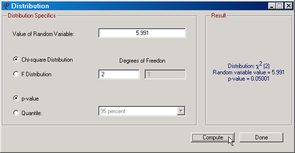
| • | Distribution: Opens the Distribution dialog from which p-values and quantile values can be calculated from the χ2 and F distributions. |
|
Figure: The Distribution dialog in SVAR.
|
Graphics Menu
| • | Cointegration Relations: Displays graphs of the cointegration relations. Available on the Toolbar. |
| • | Permanent and Transitory Components: Displays graphs of permanent and transitory components of the endogenous variables based on the multivariate Beveridge-Nelson decomposition. See, for instance, Johansen (1996), Section 5.7. Available on the Toolbar. |
| • | Residuals: Displays graphs of various features involving the reduced form residuals of the model. The first plot shows the actual data for endogenous variable along with the 1-step ahead forecast, i.e., the systematic part. The second plot gives the normalized/standardized residual, i.e., the estimated residuals divided by their estimated standard deviation. The third plot gives histograms of the normalized/standardized residuals and draws from a N(0,1) distribution. Finally, the fourth plot shows estimated partial autocorrelations for the residuals along with x percent confidence bands, where x is the selected confidence band size on the Parameters tab on the main program window. Available on the Toolbar. |
| • | Fitted Terms: Displays plots of the actual data against the estimates of various terms such as the influence of the various lagged endogenous variables in the equation, and the influence of the different cointegration relations. |
| • | Forecasting: Displays graphs of either out-of-sample or within-sample forecasts of the levels, the growth rates or both of the endogenous variables over a chosen forecast period. The graphs include point forecasts, actual values, and x percent confidence bands, where x is the selected confidence band size on the Parameters tab on the main program window. The confidence bands currently do not include uncertainty due to using estimated parameters. Available on the Toolbar. |
| • | Forecast Variable Transformation: Displays graphs of either out-of-sample or within-sample forecasts of a certain transformation of the endogenous variables over a chosen forecast period. The forecast variable can be a linear combination of two endogenous variables in levels, first differences, annual differences, and annual accumulations of the levels. This linear combination can be transformed by various functions, such as the exponential function. |
| • | Recursive Eigenvalues: Plots recursively estimated eigenvalues along with fluctuation tests based on these eigenvalues as described by Hansen and Johansen (1999). The recursive Nyblom statistics can also be plotted (see Hansen and Johansen, 1999, and Bruggeman, Donati and Warne, 2003), as well as recursive estimates of the largest non-unit eigenvalue of the companion matrix. Exactly how the recursions are performed is determined by the settings on the Recursion tab on the Preferences dialog. Available on the Toolbar. |
| • | Recursive Chow Tests: Displays plots of recursively estimated on an equation-by-equation basis, recursive sample-split and break-point tests for the system. Available on the Toolbar. |
| • | Recursive Fluctuation Test: Displays plots of recursively estimated fluctuation tests due to Ploberger, Krämer and Kontrus (1989) on an equation-by-equation basis. Available on the Toolbar. |
| • | Dummy Impulse Responses: Displays plots of the responses due to the additional deterministic variables when such are present in the model. The impulse is based on the deterministic variable being 1 in period 0 and 0 for all periods greater than 0. For models with multiple additional deterministic variables it is also possible to estimate these functions based on either long run or proportionality restrictions. |
| • | Eigenvalues of Companion Matrix: Displays a plot of the eigenvalues of the companion matrix with both their real and their imaginary part along with the unit circle itself. |
Simulation Menu
| • | Trace Distribution: Makes is possible to simulate the asymptotic distribution of the trace tests for 4 different models of the deterministics: a restricted and an unrestricted constant, and a restricted and an unrestricted linear trend. By restricted it should be understood that the parameter can be written as being equal to α times an rx1 vector of free parameters. The number of draws per replication (the length of the random walk) as well as the number of replications (number of times the statistics are calculated), the number of endogenous variables, as well as the number of exogenous I(1) variables can also be selected. The calculations are then performed as discussed by Johansen (1996), Chapter 15. |
| • | Cointegration Space Tests: Opens the dialog for bootstrapping the cointegration space exclusion, stationarity, and test on constant/trend test. See Bootstrapping the Cointegration Space Tests for details. |
Help Menu
| • | Cointegration Rank Tests: Opens the help file on this page. |
| • | Common Cycles - PDF File: Given that SVAR knows this file exists and where a PDF viewer is located on your hard drive, the PDF documentation on common cycles can be opened directly from this menu item. |
| • | Generalized Impulse Responses - PDF File: Given that SVAR knows this file exists and where a PDF viewer is located on your hard drive, the PDF documentation on generalized impulse responses can be opened directly from this menu item. |


